Identifiability: can unseen observations be recognized?¶

Here identifiability means predictive recognition of a held-out labelled observation. Mathematical identifiability of mixture fractions is a different injectivity question, explained on the mathematics page.

Scientific result¶

Full-NEON five-category mean balanced accuracy is 85.2% for unseen polygons and 73.8% for held sites. Balanced accuracy averages category recalls, so a common category does not dominate the headline. Splits keep entire GlobalID histories out of training. Labels refer to recorded polygon footprints, not verified pure material or independent annual biological truth.

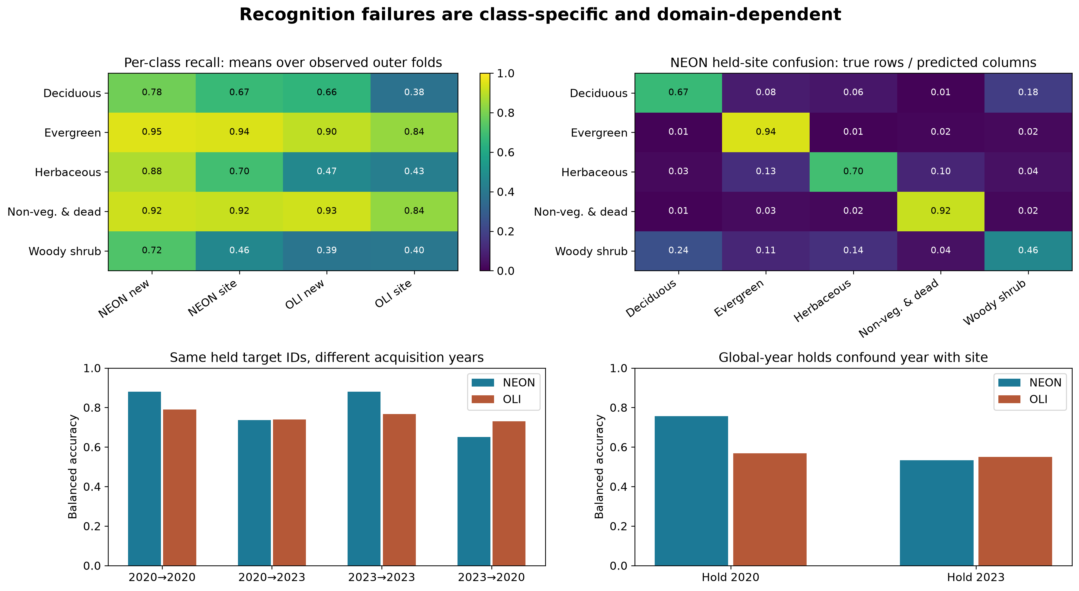
Class recalls, held-site confusion and asymmetric temporal transfer.

What you see: class-specific recognition, a normalized confusion matrix and paired/global-year evaluations. What to notice: Woody shrub held-site NEON recall averages 46.3%; Evergreen and background transfer more reliably. Paired temporal directions behave differently. What it means: the average hides important class and domain failures. What it does not mean: three sites or retrospectively reused annotations prove transfer to arbitrary regions or annual biological change. Global-year targets also change site composition; they do not isolate time alone.

How much spectral information is needed?¶

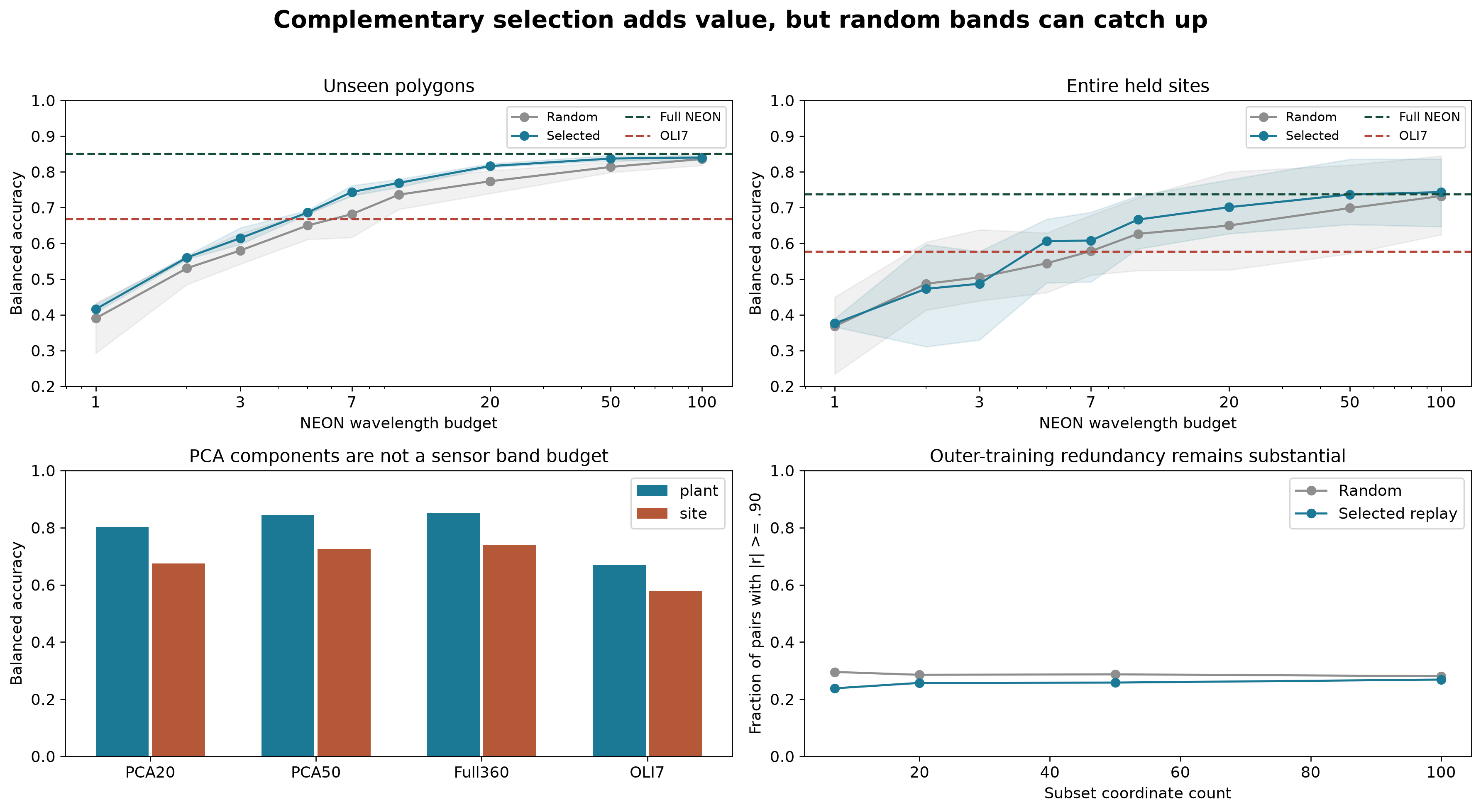
Recognition versus wavelength count for selected, random and PCA controls.

What you see: selected complementary coordinates against five fixed matched random paths, with PCA/full-spectrum comparisons. What to notice: at 20 coordinates held-site BA is 70.1% selected versus 65.0% random. Small subsets do not always win; the gap narrows at large budgets. What it means: complementary measurements add conditional moderate-budget value. What it does not mean: the selector finds universally optimal bands, the envelopes are confidence intervals, or PCA observes only its number of output components. PCA uses all input coordinates; preprocessing and selection use training data only.

Run this analysis with SpectralBridge¶

import numpy as np
from spectralbridge.library_analysis import evaluate_identifiability, evaluate_feature_budget
rng = np.random.default_rng(2)
labels = np.repeat(['A', 'B'], 18)
spectra = rng.normal(size=(36, 6)) + (labels == 'B')[:, None]
identities = np.arange(36)
result = evaluate_identifiability(spectra, labels, identities, folds=3, inner_folds=2)
curve = evaluate_feature_budget(
    spectra, labels, np.arange(500., 506.), identities,
    budgets=(1, 3), random_replicates=2, folds=3, inner_folds=2,
)
print(result['class_metrics'])
print(curve['curve'])

Pass domains=site_codes (or years) to hold out each supplied domain and purge all its identities globally. Every target class must occur in training. Insufficient inner grouped support raises an informative error; supply a single prespecified regularization=(1.,) only when tuning is intentionally unnecessary.

The output retains predictions, class-ordered scores, confusion, outer row/identity memberships, inner memberships, hyperparameters and fitted pipelines. Metrics give each identity equal total weight within a fold; fitting uses supplied rows, so aggregate or balance excessive repeated histories before fitting. Probabilities are classifier scores, not calibrated ecological uncertainty. Feature budgets are prespecified experimental settings, not chosen using the outer scores. Random paths are fixed, label-independent and nested across budgets.

Canonical primary scores, class recall and new controls retain the exact values and fold scope.