What the mathematics guarantees

A proof answers a precise conditional question. It does not certify physical calibration, field biology or every execution of a Python algorithm. The formal verification layer is separate from production execution; advanced readers can inspect the checked status matrix and illustrated report.

Preserving a mixture equation

For an ideal mixture, y = Σ fᵢ xᵢ. For the same fixed linear transformation T on the target and every reference, T(y) = Σ fᵢ T(xᵢ).

In plain language: transforming a weighted sum gives the weighted sum of the transformed components, with the same weights. Fixed convolution coefficients and fixed bandwise multipliers have this property on common finite support.

For an affine map A(x) = T(x) + b, mixture preservation also holds when Σ fᵢ = 1 (or the offset defect vanishes).

In plain language: a shared additive offset is applied once to either side when the mixture fractions sum to one. Different spatial gains, scene-fitted parameters, changing masks, clipping or hierarchical medians require separate justification. The proof does not make the complete data-dependent pipeline linear.

Preserving composition does not preserve identifiability

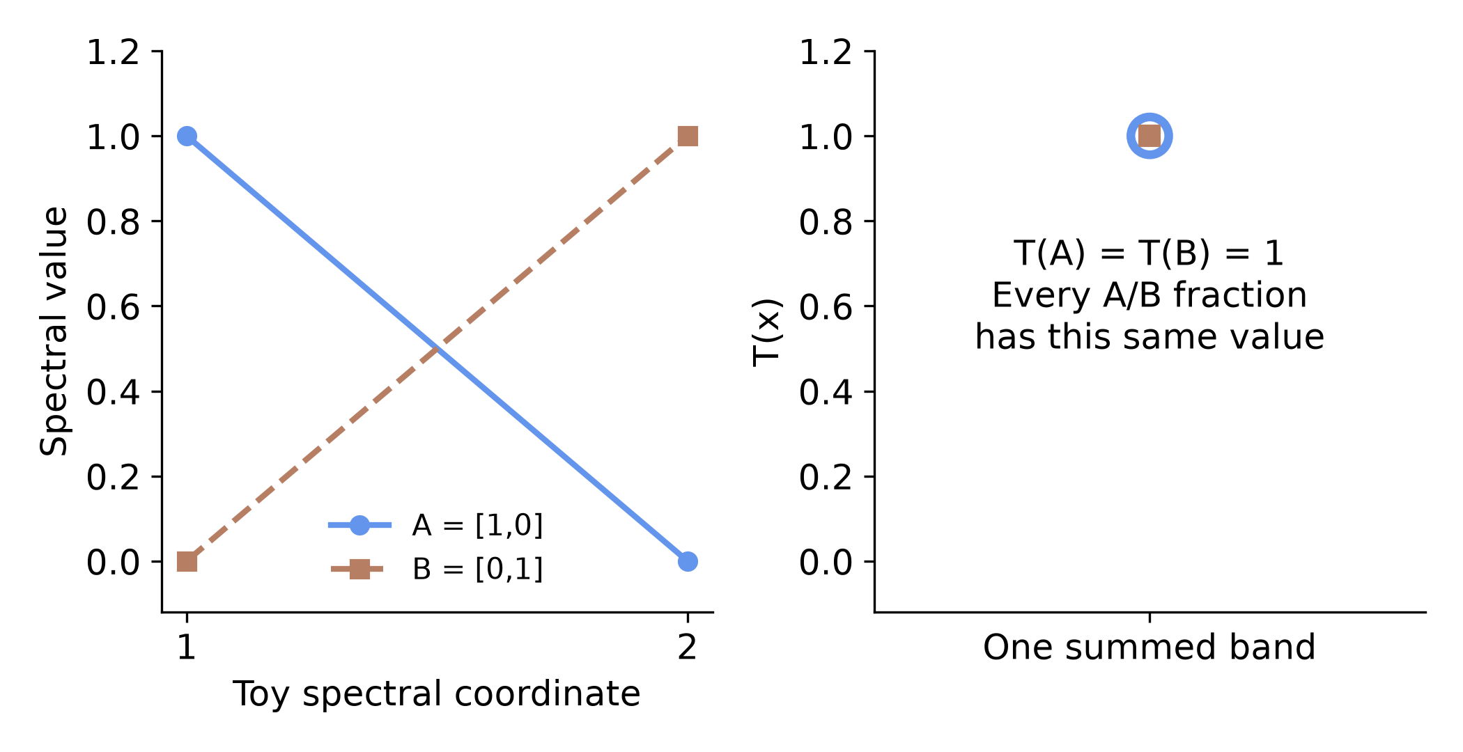
What you see: distinct hyperspectral component vectors and their reduced observations. What to notice: two distinct components map to the same measurement; mixtures still obey the transformed weighted-sum equation. What it means: algebraic preservation can coexist with lost inverse information. What it does not mean: every reduced sensor or restricted library is ambiguous. A lower-dimensional map is noninjective on the full space, but a particular restricted generating simplex can remain identifiable.

The proved example uses A=(1,0), B=(0,1) and T(x)=x₁+x₂. Both components map to 1. Every A/B mixture also maps to 1: no inverse rule can distinguish their weights from that measurement alone. A fixed linear map cannot restore distinctions that were already absent.

Solvers answer different questions

Method / claim	What is established	What is not established
Ideal FCLS	Convex objective; a minimizer exists, unique under transformed-library identifiability; known-parent recovery under stated assumptions	Every finite-tolerance Python execution or correct real biological references
Finite MESMA	Tolerance-aware selection bound over admitted finite candidates	Unrestricted exact optimization over all possible materials
Near-fit ambiguity	Restricted near-set inclusion/monotonicity; explicit counterexamples to unique composition from exact fit	Exhaustive physical uncertainty
Ridge	With fixed preprocessing and positive penalty, a unique centered coefficient minimizer per output column	Unique physical inverse or universal superiority to MESMA
Euclidean simplex projection	Valid fractions; unique projection; idempotence; no farther from a feasible truth in Euclidean error	Added spectral information, biological truth, or full formal equivalence of the Python sorting routine for every floating input

The exact-real theorems are PROVED, conditional on their explicit hypotheses. The finite rational/Python examples are NUMERICALLY CHECKED. Observed recognition and fraction scores are EMPIRICALLY SUPPORTED within the stated sampled design. These statuses must not be exchanged.

The assumption ladder

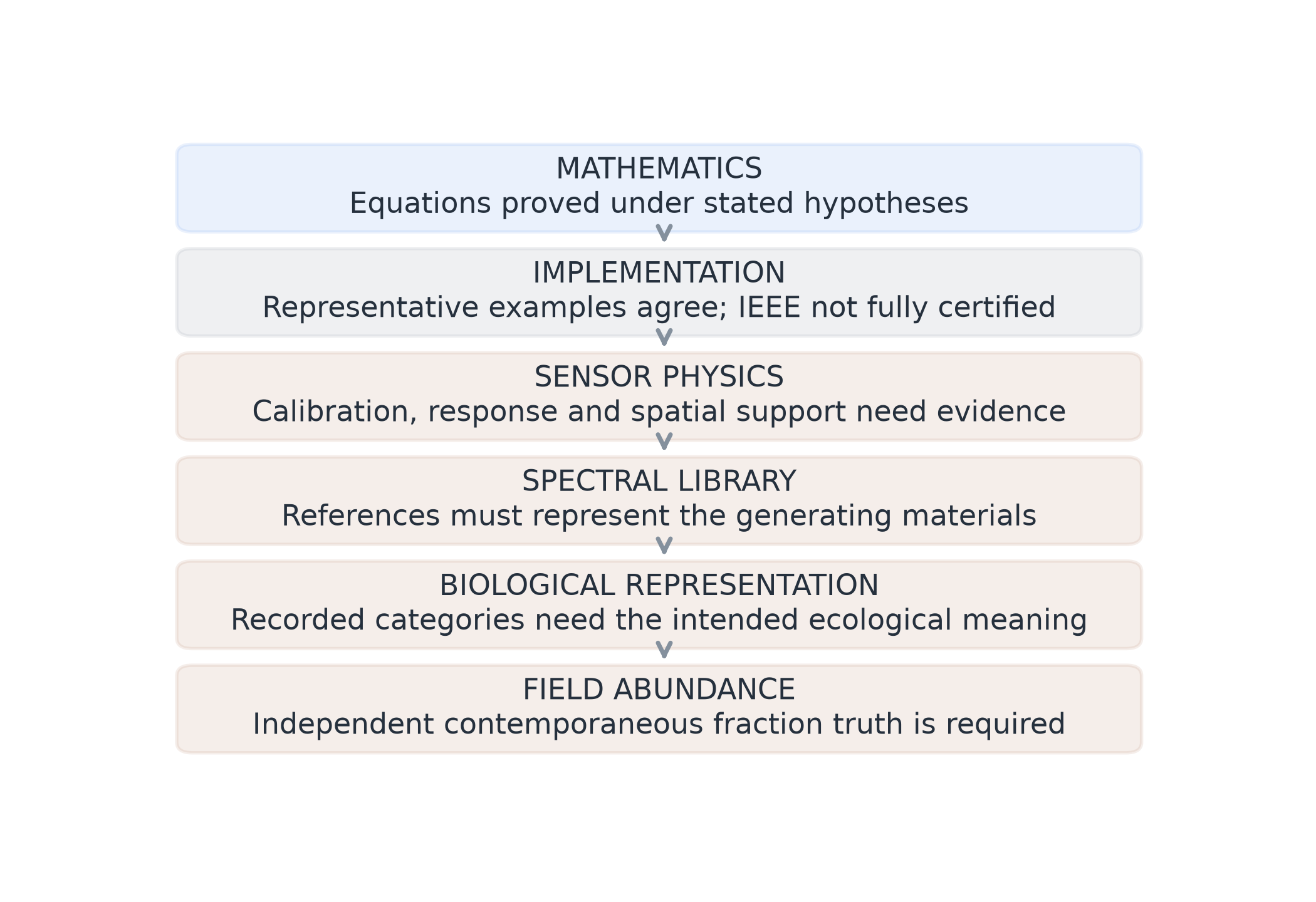
What you see: mathematics → implementation → sensor physics → spectral library → biological representation → field abundance. What to notice: each level needs evidence that the preceding proof cannot supply. What it means: proofs and observations complement each other. What it does not mean: passing one level automatically validates the next.

Level	Current status and evidence
Mathematics	PROVED / CONDITIONAL: fixed linear/affine preservation, information-loss counterexamples and ideal inference results
Implementation	NUMERICALLY CHECKED: conformance fixtures; full floating-point equivalence remains unproved and audited discrepancies remain queued
Sensor physics	CONDITIONAL: same-source response/translation arithmetic is not independent cross-platform calibration
Spectral library	EMPIRICALLY SUPPORTED / CONDITIONAL: sampled labels and held-domain experiments; adequacy for new targets is not guaranteed
Biological representation	CONDITIONAL / NOT ESTABLISHED: recorded categories do not prove pure materials, annual biological truth or correct physical mixing
Field abundance	NOT ESTABLISHED: independent contemporaneous fractional-cover validation is missing

The implementation audit includes reproduced axis-inference and overlapping extraction-window defects. Their historical scientific impact is not yet established; source lineage must be audited before regenerating results. No production fixes are part of this package/documentation expansion.

Run this analysis with SpectralBridge

from spectralbridge.library_analysis import project_simplex, candidate_ambiguity
print(project_simplex([-2., 1., .8]))  # [0., .6, .4]: valid geometry
alternative = candidate_ambiguity(
    [[1., 0., 0.], [0., .5, .5]], [0., 0.], tolerance=.01,
    class_order=['C', 'A', 'B'],
)
print(alternative['ranges'])  # exact fit can coexist with different fractions

The proof does not tell us that every abundance estimate is true. It tells us precisely what must be true for an abundance estimate to have the interpretation we give it.